
The Laplace transform technique becomes truly useful when solving odes with discontinuous or impulsive inhomogeneous terms, these terms commonly modeled using Heaviside or Dirac delta functions. We will discuss these functions in turn, as well as their Laplace transforms.
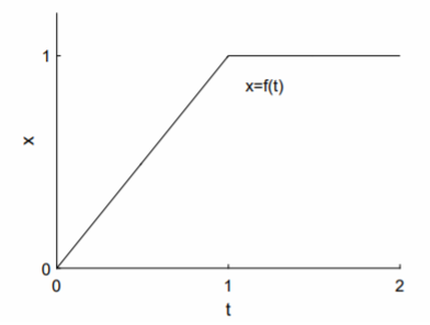
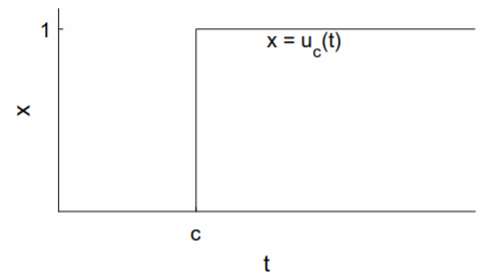
View tutorial on YouTube The Heaviside or unit step function (see Fig. \(\PageIndex\)) , denoted here by \(u_c(t)\), is zero for \(t \[\labelu_c(t)=\left\0,&t\right.\] The precise value of \(u_c(t)\) at the single point \(t = c\) shouldn’t matter. The Heaviside function can be viewed as the step-up function. The step-down function—one for \(t \[\label1-u_c(t)=\left\1,&t\right.\] The step-up, step-down function—zero for \(t \[\labelu_a(t)-u_b(t)=\left\0,&t\right.\] The Laplace transform of the Heaviside function is determined by integration: \[\begin\mathcal\&=\int_0^<\infty>e^u_c(t)dt \\ &=\int_c^<\infty>e^dt \\ &=\frac>,\end\] and is given in line 12 of Table 5.1.1. The Heaviside function can be used to represent a translation of a function \(f(t)\) a distance \(c\) in the positive \(t\) direction. We have \[u_c(t)f(t-c)=\left\0,&t\right.\nonumber\] The Laplace transform is \[\begin\mathcal\&=\int_0^<\infty>e^u_c(t)f(t-c)dt \\ &=\int_c^<\infty>e^f(t-c)dt \\ &=\int_0^<\infty>e^f(t')dt' \\ &=e^\int_0^<\infty>e^f(t')dt' \\ &=e^F(s),\end\] where we have changed variables to \(t' = t − c\). The translation of \(f(t)\) a distance \(c\) in the positive \(t\) direction corresponds to the multiplication of \(F(s)\) by the exponential \(e^\). This result is shown in line 13 of Table 5.1.1. Piecewise-defined inhomogeneous terms can be modeled using Heaviside functions. For example, consider the general case of a piecewise function defined on two intervals: \[f(t)=\left\f_1(t),&\textt
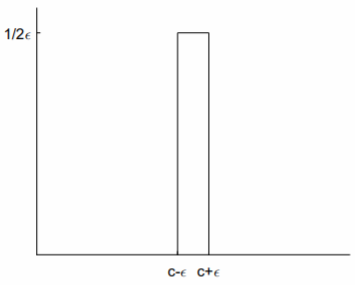
View tutorial on YouTube The Dirac delta function, denoted as \(\delta (t)\), is defined by requiring that for any function \(f(t)\), \[\int_<-\infty>^<\infty>f(t)\delta(t)dt=f(0).\nonumber\] The usual view of the shifted Dirac delta function \(\delta (t − c)\) is that it is zero everywhere except at \(t = c\), where it is infinite, and the integral over the Dirac delta function is one. The Dirac delta function is technically not a function, but is what mathematicians call a distribution. Nevertheless, in most cases of practical interest, it can be treated like a function, where physical results are obtained following a final integration. There are many ways to represent the Dirac delta function as a limit of a welldefined function. For our purposes, the most useful representation makes use of the step-up, step-down function of \(\eqref\) (see Fig. \(\PageIndex\)): \[\delta(t-c)=\underset<\lim>\frac(u_(t)-u_(t)).\nonumber\] Before taking the limit, the well-defined step-up, step-down function is zero except over a small interval of width \(2\epsilon\) centered at \(t = c\), over which it takes the large value \(1/2\epsilon\). The integral of this function is one, independent of the value of \(\epsilon\). The Laplace transform of the Dirac delta function is easily found by integration using the definition of the delta function: \[\begin\mathcal\&=\int_0^<\infty>e^\delta (t-c)dt \\ &=e^.\end\] This result is shown in line 14 of Table 5.1.1.
This page titled 5.3: Heaviside and Dirac Delta Functions is shared under a CC BY 3.0 license and was authored, remixed, and/or curated by Jeffrey R. Chasnov via source content that was edited to the style and standards of the LibreTexts platform.